Notebook Editor
Each user experiment or study is described in a notebook, an advanced form of hypertext that combines text and data with its processing and visualisation. Once opened, a notebook looks like a real paper notebook:
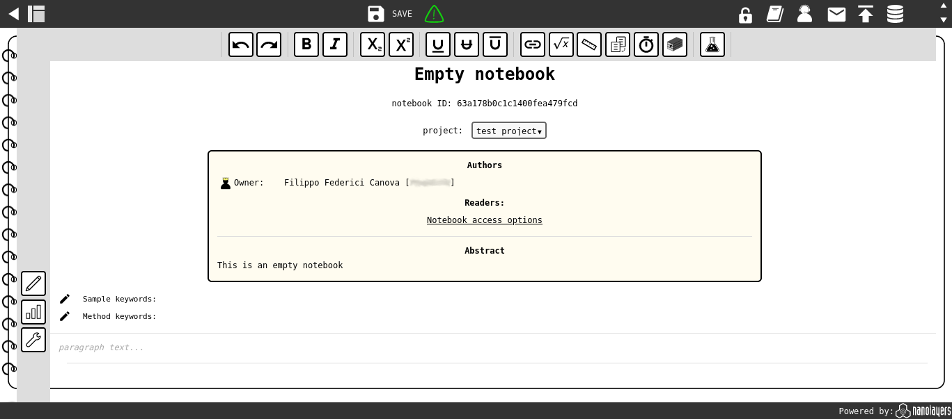
An empty notebook.
The notebook page shows the title, a header, and the notebook content. The header shows a list of authors, editors and readers that have access to the notebook, followed by the abstract, and finally the notebook content (initially empty). Start editing the notebook by clicking on the placeholder text and typing, or by adding Notebook Elements.
Notebook Access Control
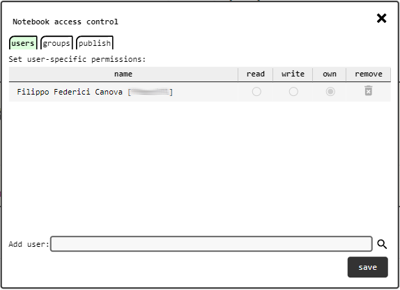
Notebook access control panel.
Initially only the user that created the notebook (its owner) is listed in the authors. Permissions for other users and groups can be changed in the access control panel, which opens by clicking on the notebook access control link above the abstract area.
NavBar
The NavBar is always displayed at the top of the display area, showing the following buttons and indicators:
 - return to the Dashboard
 - Save the notebook and abstract as they are on screen
 - notebook Sanity Check (button and indicator)
 - user lock (indicator)
 - open this documentation
 - open the help request panel
 - open the Messaging System panel
 - open the Data Uploader panel
 - open the Data Explorer panel
 /
/ - quickly navigate to beginning/end
Warning
The system saves exatly what appears on screen. If, for any reason, there is an error/bug and the notebook fails to load completely, DO NOT click the save button as this will overwrite your notebook with the partially loaded one. In such case, refresh the page and, if the problem persists, contact the system administrators.
Save the notebook
The ![]() button in the navbar saves both abstract and notebook content, as they appear on screen, in the platform database.
button in the navbar saves both abstract and notebook content, as they appear on screen, in the platform database.
Note
Save frequently in order to avoid losing your work!
Warning
The system saves exatly what appears on screen. If, for any reason, there is an error/bug and the notebook fails to load completely, DO NOT click the save button as this will overwrite your notebook with the partially loaded one. In such case, refresh the page and, if the problem persists, contact the system administrators.
Sanity Check
The sanity check detects inconsistencies between the notebook version stored in the database and the one visible in the browser. An inconsistency is usually the result of notebook edits saved in a different browser tab, possibly by a different user, that were not loaded in the current user session.
When this occurs, the system will inform the user that the notebook version being displayed does not match the one found in the database. The user is prompted to refresh the notebook, losing any of their unsaved changes, or carry on, overwriting the database version with their own when saving, and thus losing the external edits.
The check is performed automatically and periodically while the notebook is open, however, clicking the ![]() button in the navbar will manually trigger a check.
button in the navbar will manually trigger a check.
Note
It is always best to avoid concurrent edits. Restrict other users to read-only access unless necessary.
Messaging System
This panel shows a log with all messages, their sender and timestamp, and lets users send send new messages to all users that have access to the notebook (optionally also via email).
Note
Only users with explicit permission will receive the message via email. Users with read access through their group will not get the email but can see the message in the log.
Text Editing Toolbar
When the cursor is placed into an editable text area (any paragraph, section header or caption), the text editing toolbar will appear below the NavBar:

The first two are the standard undo (![]() ) and redo (
) and redo (![]() ) buttons.
) buttons.
The next seven buttons are text style controls, also commonly found in many text editors:
 bold
bold italic
 subscript
 superscript
 underline
 strike through
 overline
These style controls can be independently turned on/off by clicking the corresponding button. If a text selection is in place, the style will be applied to the selection. If a normal cursor is placed instead, the style is applied to the next entries.
Note
Some styles may not take effect when applied to section headers.
The last group of buttons are inline elements:
Clicking on one of these will insert the corresponding inline element at the cursor position in the notebook.
Some inline elements are simple and can be edited in the notebook by clicking on them. Some are more complex and hovering the mouse pointer on them will show a configuration button (![]() ) that opens a dedicated panel with their settings.
) that opens a dedicated panel with their settings.
Note
Some inline elements might not be available when editing the notebook abstract.
Inline Elements
Inline elements appear inside text containers (paragraphs, captions, …) to add small, special features such as citations and references. These are added in the text at the cursor position when clicking the corresponding button in the Text Editing Toolbar.
 External Links

A link as it appears after being inserted.
This inline element creates a link to an external URL. When the mouse pointer is over the element, a small control button will appear: this opens the configuration panel to setup the link destination URL and the text to be displayed. Clicking the actual text of the link will redirect the browser to the given URL, just like a normal link.
 Inline Math
Inline math as it appears after being inserted.
When a new inline math is added, it shows the default x=0 expression. Clicking on it will show a text area for the LaTeX code. After editing, defocus the element (click away) and the text area will disappear, leaving the rendering of the LaTeX source code.
Note
The platform uses MathJax to render all maths expressions in the notebook, so it is limited to its capabilities.
 Physical Quantity

Physical quantity as it appears after being inserted (left) and after setting it non-verbose display with physical units (right).
This inline element offers a convenient way to represent quantities with units. When added, a physical quantity uses symbol q and value 0. Click the quantity to open the configuration panel and change its settings:
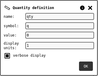
Configuration panel of a physical quantity.
The editable fields are:
name: internal name of the quantity (not used yet)
symbol: LaTeX expression to use as visual name of the quantity
value : string with the value and physical units
display units: units to use in the rendered expression
The value will be converted to the given display units without changing the original value stored in the notebook.
Verbose display shows the quantity as symbol = value, while non-verbose display only shows value.
 Cross-References
Certain elements in the notebook can be cross-referenced, thus creating a quick link between text and visual elements. When added, a new cross-reference will show as a red placeholder until it is set to target a referrable item in the notebook using its configuration panel: pointing the mouse on the cross-reference will reveal the button to access the panel.
Referrable elements are:
section
figure
table
script
structure
Note
Several elements are referred to as figure: images and all kinds of plots.
Once the cross-reference target is set, clicking it will act as an internal link, scrolling the page to bring the target element into view.
 Timestamps
Timestamps can be useful to keep track of when certain steps occurred during an experiment.

Example timestamp.
A timestamp will always show the time when added into the text as it was on the client system. The interface will convert automatically the timestamp to the client’s timezone. It is possible to change the time display format in the configuration panel.
Warning
There is no way to change the actual timestamp using the interface.
 Bibliography
This element brings citations into the notebook text, often targetting articles in scientific journals, books or conference proceedings.
An empty citation added to the text can be configured from its configuration panel. The upload tab is used to insert bibliography elements from bibtex files into the AMAD database, with a simple drag and drop interface. All definitions found in the dropped files will be parsed and uploaded.
Note
The bibliography database is global: all users can see and use references uploaded by any other user.
Warning
There currently is no check for duplicate entries. Please run a search before uploading a bibtex file, and report duplicates to the system administrators.
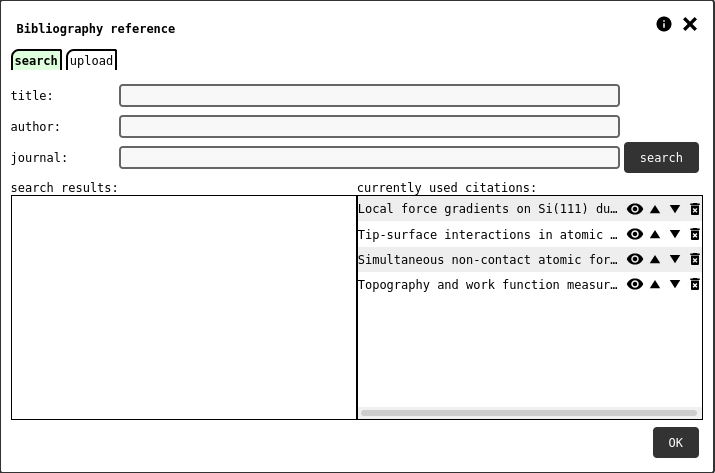
search tab of the bibliography configuration panel.
Citations can be looked up in the search tab and added to the bibliography element. The interface will display a Bibliography section at the end of the notebook, automatically generated from all citations added to the notebook.
 Inventory Interaction Element
This element allows users to interact with the Inventory Management System, by specifying in the notebook text that a particular item has been used.
Initially, the text element is empty, and it has to be configured with its configuration panel (accessed by clicking on the element).
The possible targets for the element are all items from all the labs where the user is a member.
If the target item is a consumable, the user can set the exact amount used.
Sidebar
The sidebar also appears after clicking in the abstract or notebook areas, and is used to insert new Notebook Elements into the document, such as tables and figures. The elements are sorted into different categories, therefore the sidebar needs to be navigated to find the desired element. Initially the sidebar shows the main menu with the three element categories:
After opening one of the categories, the ![]() button brings the sidebar back to the main menu.
button brings the sidebar back to the main menu.
Notebook Elements
Notebook elements are the basic building block of a notebook, such as sections, paragraphs, figures and tables. These can be dragged from the Sidebar and dropped into the notebook where they are needed. While dragging an element, special markers will appear in the notebook at valid placement locations where the element can be dropped.
Note
Some elements have placement restrictions, e.g. sub-sections are only allowed within a section.
Alternatively, it is also possible to click the new element button in the sidebar in order to place it at the current cursor location.
Note
Placement via click is only possible after the user has clicked in some notebook text area, thus placing the caret.
Elements that require user actions to configure their appearence will prompt their configuration panel (![]() ) immediately when they are added into the notebook.
) immediately when they are added into the notebook.
Most elements appear as blocks with a dedicated toolbar in the top-right corner when the mouse pointer is overing them:
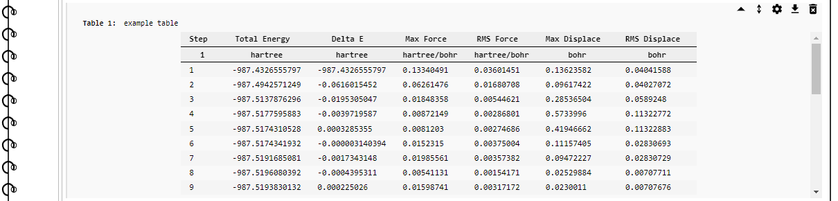
Example of a table element. The toolbar in the top-right corner appears when the mouse pointer is over the element area.
The control buttons in the toolbar common to most elements are:
- / fold/unfold element
 hold click and drag to move the element to a new location
 open the configuration panel
 download the content of the element
 delete the element
Some elements may have special control buttons that will be discussed in their respective sections.
Note
Deleting the element will not delete any data records that were uploaded or visualised in the element itself.
 Text Elements
Text elements are basic building blocks of the notebook. The first four are used to give the text a hierarchical structure:
 section
 sub-section
 sub-sub-section
 text paragraph
These elements have some placement restrictions; for example, sections can only be placed in the notebook body, while sub-sections can only go inside sections. Sections are automatically numbered. Text paragraphs are the main text containers and ca also be added to the notebook by pressing Enter when the cursor is in any editable text in the notebook.
Other elements are:
 image element - visualise/draw images
 display a LaTeX math expression
 bullet points list
 numbered list
Lists can be nested into each other, but cannot contain any other element except list items (created by pressing Enter) or other lists. These elements are quite self-explanatory, however the image block requires more complex user interaction to work and will be documented in the next section.
Image Element
The image element brings pictures into the notebook. The element consists of a chosen image, centered in the page, and a caption. The element is automatically numbered and labelled as Figure X. The configuration panel has two tabs: select and draw.
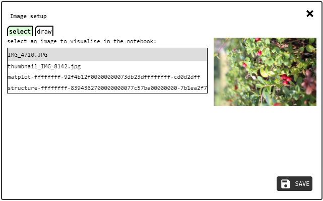
select tab of the image configuration panel.
The select tab lets the user chose one of the existing IMAGE records to be visualised in the element. Simply click the desired image and a preview will appear next to the image list. Then press the OK button to save the selection and close the panel.
Note
IMAGE records are uploaded into the notebook through the Data Uploader panel.
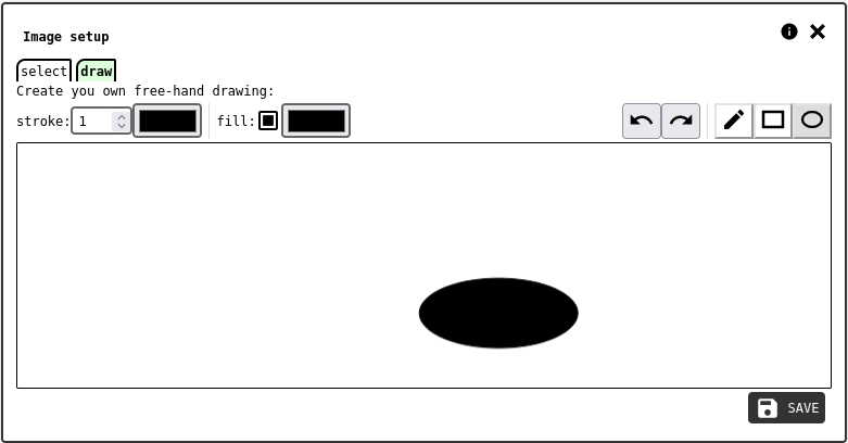
draw tab of the image configuration panel.
The draw tab is a simple drawing tool to make sketches and save them as IMAGE data records.
 Data Visualisation Elements
These are the currently available data visualisation elements in AMAD:
 table
table active table
 line/scatter plot
 histogram
 2D plot
 custom matplot (matplotlib python script)
 NMR data plot
 atomic structure
 chemdraw
Most data visualisation elements allow the user to visualise and/or create data records of a specific type from their configuration panel (![]() ).
).
Table Element
The table element lets the user visualise multiple DATA1D records in a tabular format. Each column will be displayed with two header rows for the record name and physical units.
The configuration panel (![]() ) upload tab is used to parse table files (CSV ot NPY) into DATA1D records, and upload them to the server:
) upload tab is used to parse table files (CSV ot NPY) into DATA1D records, and upload them to the server:
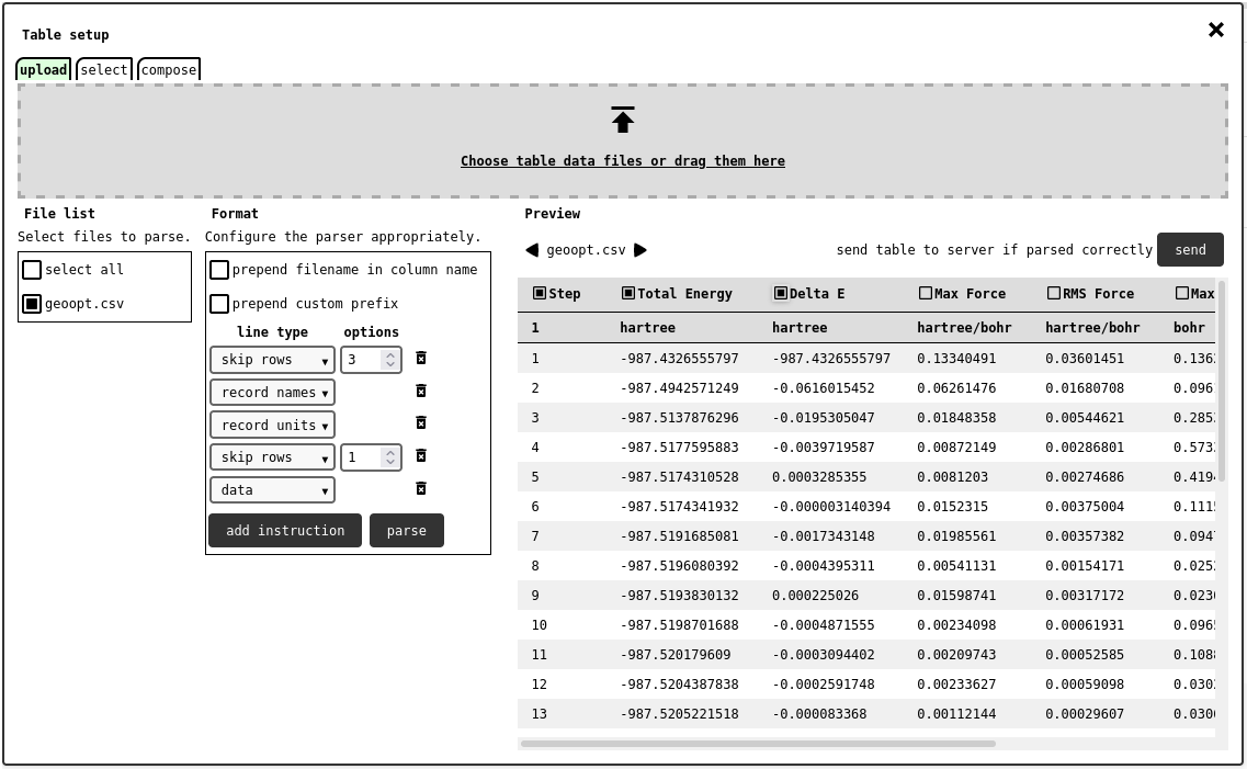
upload tab of the table configuration panel, showing how to configure the CSV parser to skip comment lines and interpret header lines.
The files drop in the designated are will be shown in the list of the left side of the panel, each with a checkmark selector: one or more files can be marked for parsing this way. Due to the heterogeneous nature of CSV formats, the user will be asked to provide the general structure of the file using the format panel. The parser will proceed in a line-by-line fashion, following the given instructions:
instruction |
function |
|---|---|
record names |
next line contains names for each column |
record units |
next line contains physical units for each column |
skip row (n) |
the next n lines will be ignored |
data |
data rows from the next line, to the end of file |
Note
Parser instructions are ignored for numpy arrays and matrixes in NPY files.
Note
A similar parse and upload interface is available in the Data Uploader panel, however this one is more flexible as it allows the user to select which columns to upload.
If the files are NPY or do not have a header that can be used record names, they will be automatically assigned. The use can opt to prepend the file name and/or custom text prepended to the record names: this is useful when uploading repeated experiment results. If records units are not specified, the system will assign 1 (adimensional) to the records: units can be edited after uploading the data from the Data Explorer.
The preview area will show the parser results for each file marked for parsing, and report eventual errors. If the preview does not look right, there could be a mistake in the parser configuration, or the data file itself could be corrupted. Otherwise, the user should select the columns to upload using the checkbox next to each previewed column and click the send button to upload the desired columns to the server as DATA1D records.
Once DATA1D records have been uploaded, the user can configure the table to visualise in the notebook from the select tab:
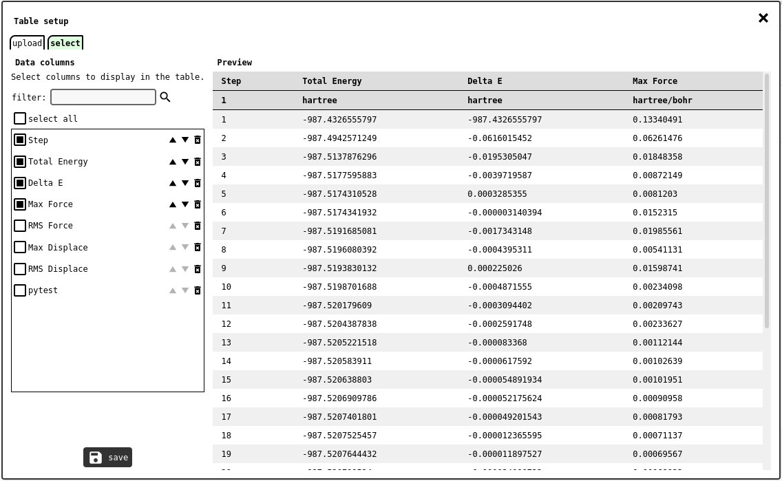
select tab of the table configuration panel.
Selectors for all DATA1D records uploaded into the notebook will be listed on the left, while the ones marked by the user will be displayed in the preview area. The order of the chosen records can be modified with the control buttons on each record selector (![]() /
/![]() ). Finally, click on the save button to store the table configuration into the server and close the configuration panel.
). Finally, click on the save button to store the table configuration into the server and close the configuration panel.
Active Table Element
The active table is a more flexible version of the Table Element, where each table cell is an independent entry, stored as a DATA0D record.
This element is designed to be a part of an active learning workflow, hence there are several Python API tools dedicated to access and manipulation of active tables (see here), so that users can apply their own machine-learning methods.
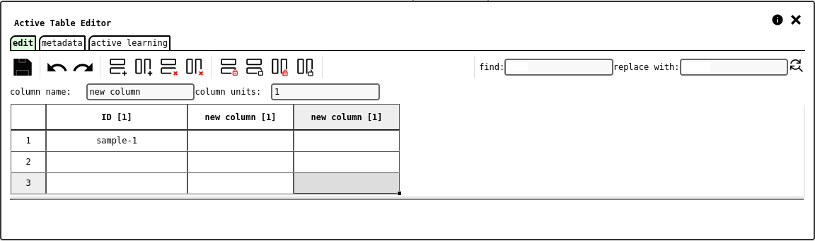
edit tab of the active table configuration panel.
The edit tab consists of an intuitive table editor, with extra controls to create and configure columns, as well as lock columns or rows to prevent edits. The interface supports copy/paste from Excel.
Note
The ID column is technically not part of the data table, as it is used as header for each row. Typically this column contains a sample identifier, while the data columns list its chemical/physical properties.
Note
The system automatically converts cell content to numbers when possible, assuming . (dot) as the decimal separator.
The tool bar buttons are:
- : save the table as it appears in the editor
 : undo last table edit
 : redo last undone table edit
 : insert a row before the selected one
 : insert a column before the selected one
 : remove selected rows
 : remove selected columns
 /
/ : lock/unlock selected rows
 /
/ : lock/unlock selected columns
Finally there is a simple control to perform find/replace operations in text cells. This can be particulary useful to replace wrong decimal separators, or remove unwanted symbols.
Note
Some tool buttons might be disabled if the user selection does not allow the operation.
Underneath the main tool bar, there is a secondary control panel to set the name/units of the selected row or column.
Note
This secondary controls might be hidden if the user selects multiple rows or columns.
The metadata tab is used to set row- and column-wise metadata tags for the table. The DATA0D records associated with each cell will get labelled automatically according to these specifications. This will make it easier to compile datasets.
The active learning tab shows the controls to perform machine learning operations (server-side) and display results.
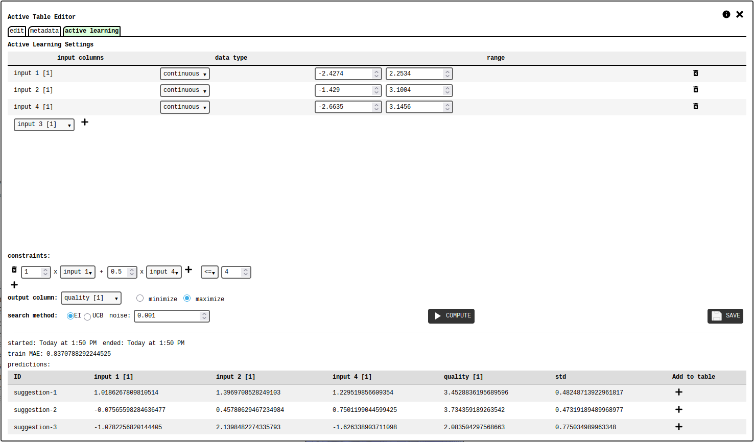
active learning tab of the active table configuration panel.
The user must select the table columns to use as input features and their numerical ranges. The data type of each column can be:
continuous: any real value within the specified range
integer: any integer value within the specified range
discrete: any of the comma-separated values given in the range field
categorical: any of the comma-separated entries given in the range field
Note
When selecting discrete or categorical, the system autofills the range with values found in the respective column.
Note
All data types for input columns assume numerical values, except categorical which treats all column entries as text.
Warning
Predictions for categorical inputs are limited to only entries found in the table. If new category labels, not found in the actual table column, are added to the range field, the system will not be able to infer their relationships with the available ones.
Additionally, it is possible to add linear constraints to the search space. For example, this can be used in materials research to enforce physically meaningful compositions, or experimental limitations.
One data column has to be chosen as the optimisation target, and it is necessary to select whether to perform minimisation or maximisation.
Possible search methods are: * EI (Expected Improvement): favors points closer to maxima/minima * UCB (Upper Confidence Bound): favors exploration
The user must also provide a noise value.
Clicking the COMPUTE button submits the settings and initiates the calculation on the server, which uses gaussian processes to model the relationship between the inputs and the output. When completed, the tab will display a list of suggested input sets, one of which is the expected best candidate. The user can add any of the suggestion to the active table.
Line/Scatter Plot Element
The line/scatter plot element provides simple plotting capabilities into the notebook. The configuration panel (![]() ) is used to setup the plot:
) is used to setup the plot:
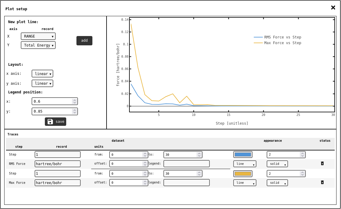
line/scatter plot configuration panel.
In order to add new traces to the plot, select the appropriate DATA1D records to use on the x and y axes with the selectors in the top-left side of the panel, then click the add button. The number of entries in the x and y data records have to match, or the system will show an error. All traces will appear in the lower part of the panel, with several controls to adjust their appearence.
The from/to fields determine the index of the first/last trace point to show in the plot: these let the user prune the data range of the records. Negative numbers indicate indexes from the end of the trace: -1 being the last point, -2 the one-to-last.
The offset value applies a user-defined vertical shift to the trace.
The legend field can be used to override the automatic legend text for the trace.
The appearence controls (color, thickness, trace type, line type) are self-explanatory.
It is also possible to specify custom physical units for each data record used in the plot. This will perform a unit conversion on-the-fly, if the given units are compatible with the ones originally assigned to the record.
Note
This is not altering the data in the database, just the way it is visualised.
Any change to the plot settings will trigger an update of the preview panel (top-right), or display an error. Additional layout controls for legend position and axes types are found in the left panel. Once the plot is setup, click the (![]() ) save button to confim the settings and close the configuration panel.
) save button to confim the settings and close the configuration panel.
Note
The plot is saved and visualised in the least memory-intensive way. If the data records used to make the plot are not too large, the notebook will show an interactive plot made on-the-fly, like the preview one in the configuration panel. Otherwise, the plot will be saved as an IMAGE record in either SVG, PNG or JPEG format, and visualised in the notebook as a static picture.
Warning
If the units of any trace source data are changed, the plot axes labels might not automatically change. The trace should be removed and added again to the plot after the units changed to get the connect labels.
Histogram Element
With this element the user can create histograms from uploaded DATA1D records.
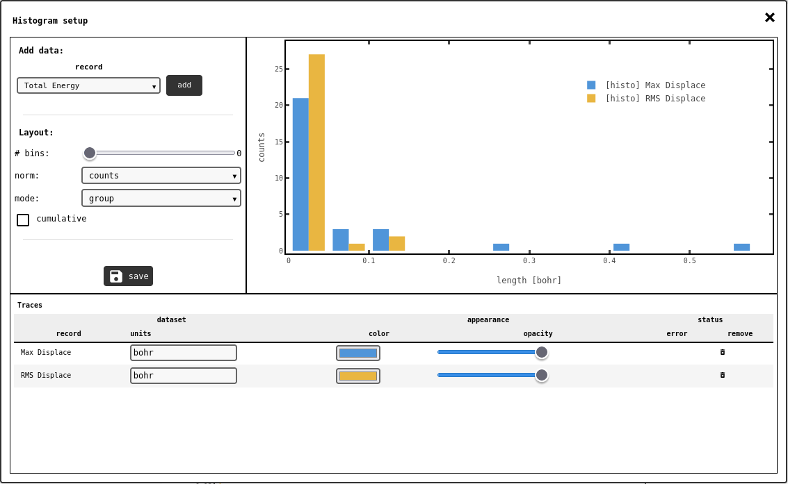
Histogram configuration panel.
The interface is similar to the line/scatter plot configuration panel: select the DATA1D record in the drop-down selector (top-left) and click the add button. The entries in the data record will be automatically binned: use the # bins slider sets the total amount of histogram bins to generate, or set to zero/auto to let the system’s heuristics decide.
Normalisation method (norm) and charting mode (mode) can also be set in the drop-down selectors on the left.
When the histogram is setup correctly, click the (![]() ) save button to accept changes and close the panel.
) save button to accept changes and close the panel.
2D Plot Element
This element is intended to plot two-dimensional data (DATA2D) either in a heatmap or contour plot fashion.
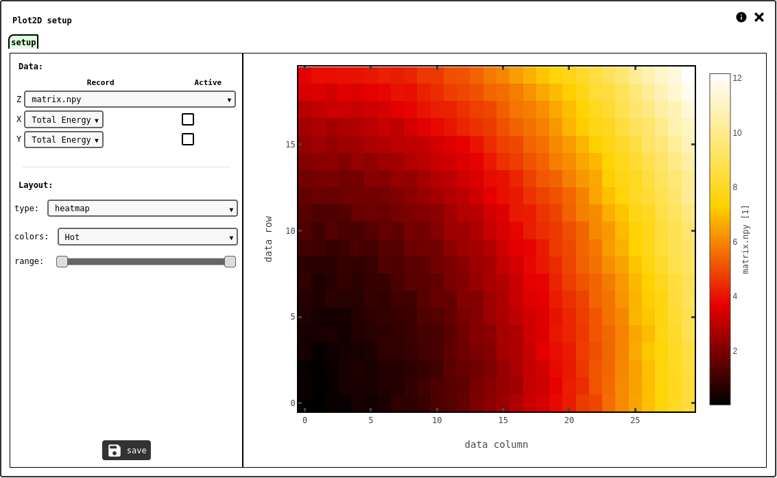
setup tab of the 2D plot configuration panel.
The DATA2D record to plot should be selected in the drop-down selector for the Z axis. By default the x/y axes are just the column/row index if each matrix element, but it is possible to assign specific values for these axes from DATA1D records: set the corresponding record selectors and mark the checkboxes to use the custom records as x/y axes values. The size of the DATA1D records used for the plot axes have to match the shape of the DATA2D record on Z, or the system will report an error.
The layout options let the user chose the plot style (heatmap or contour), in a variety of pre-defined color scales.
Custom MatPlotLib Element
The most advanced plotting tool in AMAD lets the user create custom plots using special python scripts.
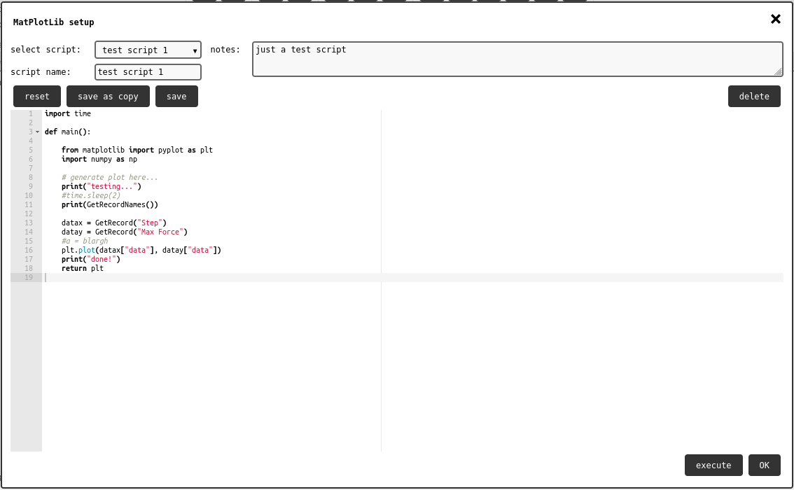
Matplot element configuration panel.
The configuration panel shows a list of exising scripts, with the option to create a new one. Once a script is selected, it is possible to edit its info text, and check the source code in script editor showing in the main portion of the panel.
The save button saves the current script: if this was used somewhere else in the notebook (or in a different notebook), the changes will be applied everywhere.
Warning
Saving a script used somewhere else will not trigger a re-run of the script, so any result will not be lost (although the script will be).
The save as copy button saves the current source code to a new script, thus not replacing any pre-existing script.
The reset button clears the source code and sets it to the default empty script.
The delete button will remove the selected script from the system.
Warning
the script will be deleted even if it is used somewhere else.
As seen in the default script, the main function has to return the pyplot object from matplotlib. It is up to the user-defined code to set it up appropriately with the desired plot. Check the Scripting Guidelines for more info about scripting.
Scripts are queued for execution using the execute button in the configuration panel, or in the element toolbar (![]() ). Once execution is finished on the server, the element will be updated with the resulting plot, or an execution log if errors occurred. It is always possible to check the execution log with the script screen output using the
). Once execution is finished on the server, the element will be updated with the resulting plot, or an execution log if errors occurred. It is always possible to check the execution log with the script screen output using the ![]() control button.
control button.
Nuclear Magnetic Resonance
NMR data records (see NMR / Bruker) can be visualised in the notebook with this element.
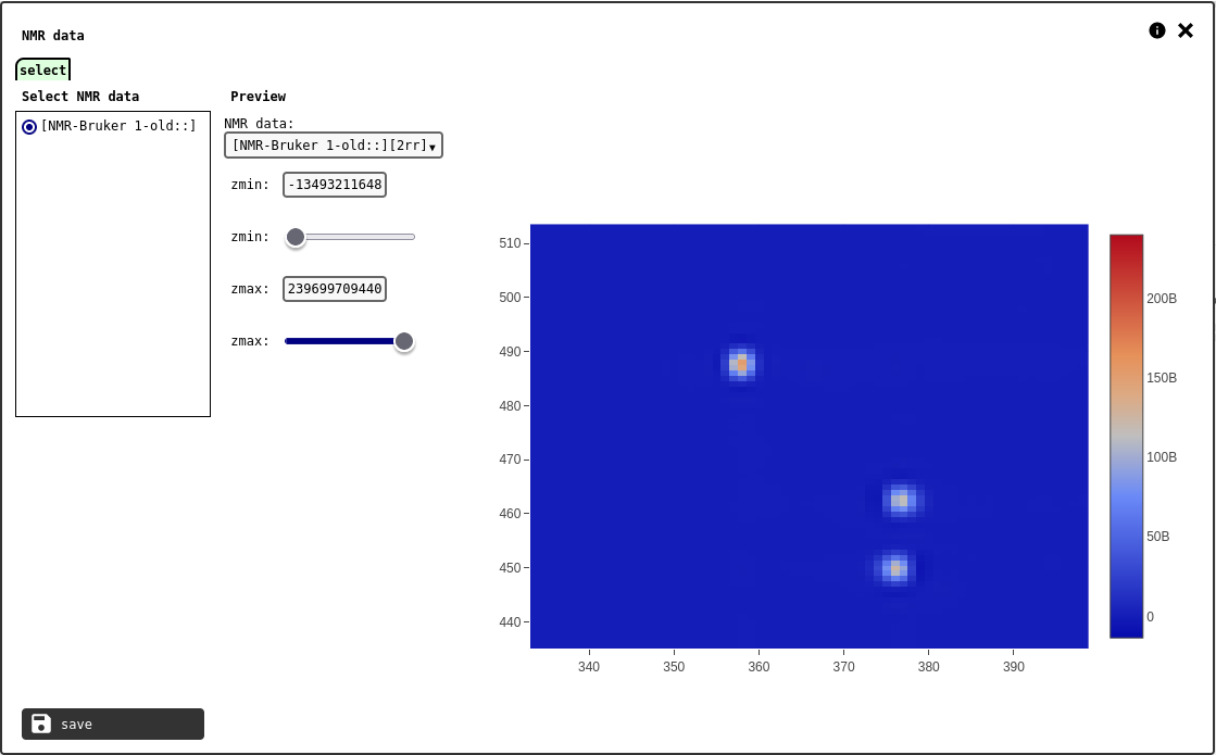
select tab of the NMR element configuration panel.
The interface has a channel selector and sliders to tweak the data range.
Atomic Structure Element
STRUCTURE records can be visualised in the notebook using this element. The select tab can be used to chose one to display in the element.
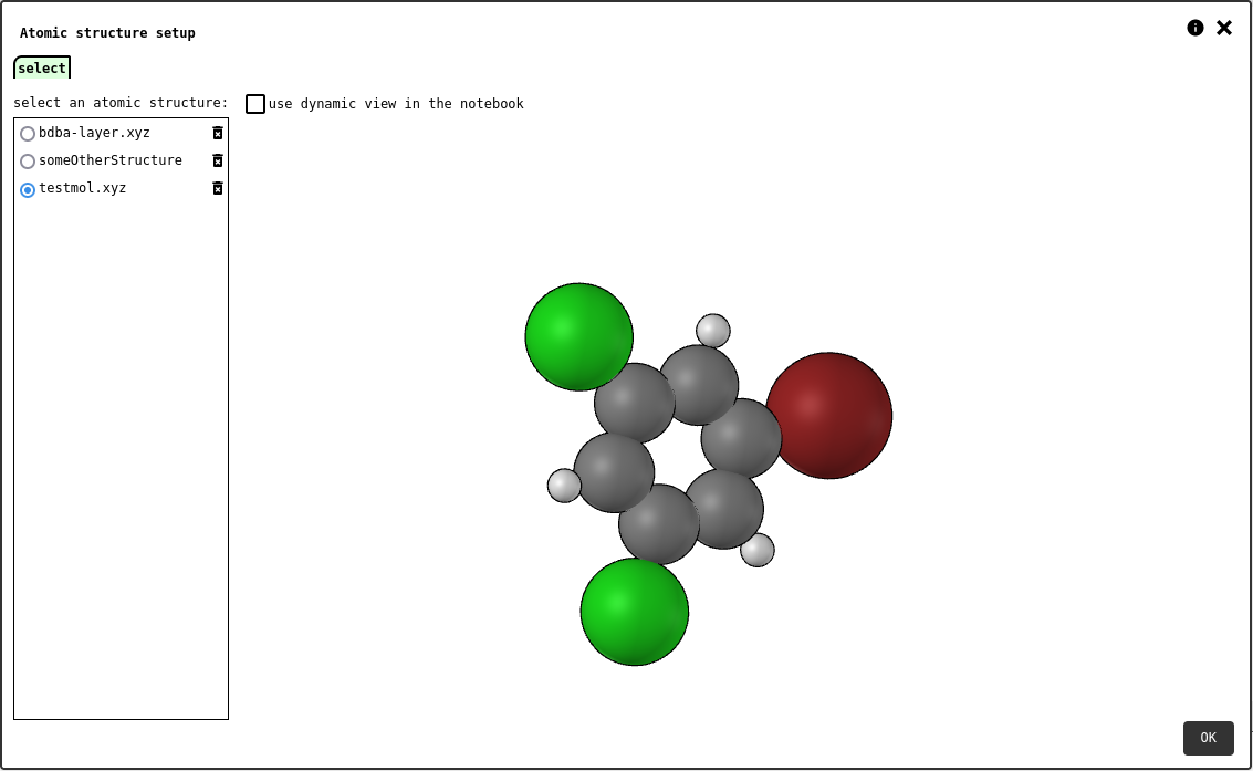
select tab of the atomic structure element configuration panel.
If the dynamic mode option is checked, the notebook element will display an interactive atomic structure viewer that lets any reader rotate/pan/zoom the chosen molecule at will. Otherwise, the system will take a snapshot of the preview and store it as an IMAGE record that will be statically displayed in the notebook element.
The ![]() control button in the element toolbar toggles the atomic coordinate panel (XYZ format).
control button in the element toolbar toggles the atomic coordinate panel (XYZ format).
ChemDraw
This element is used to create and visualise chemdraw representations of molecules or reactions. The chemdraw can be generated from SMILES, loaded from a file, or designed by the user.
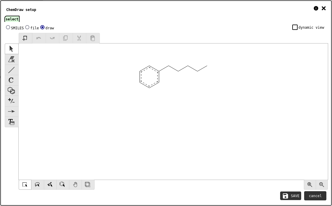
select tab of the chemdraw element configuration panel showing the designer interface.
If the dynamic mode option is checked, the notebook element will display an interactive viewer that lets any reader pan/zoom the chemdraw at will. Otherwise, the system will take a snapshot of the preview and store it as an IMAGE record that will be statically displayed in the notebook element.
Note
Chemdraws are not stored as data records.
 Data Processing Elements
These elements are tools for processing data uploaded into the notebook. The processing output is usually stored as new data records, but some elements also create plots.
 Principal Component Analysis
Principal component analysis (PCA) is a widely adopted data analysis tool, often used for dimensionality reduction, data visualisation as well as to extract information from large, complex datasets.
Essentially, it is a linear transformation of the data, so that the directions (principal components) capturing the largest variance in the data can be easily identified.
The notebook element allows the user to select a data source, compute the principal components and generate a 2D or 3D plot using any combination of desired components.
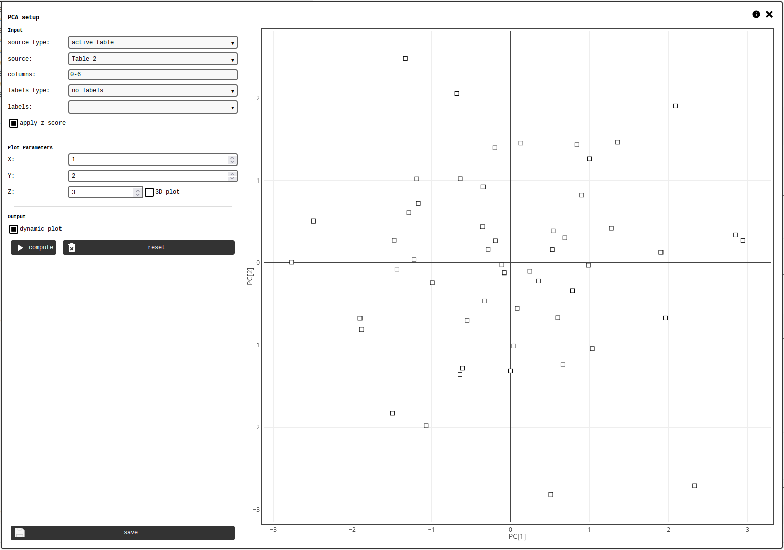
PCA element configuration panel.
The calculation requires any kind of matrix-like data, and optionally a vector-like with labels. The data should be organised so that each row of the matrix describes one data point. The data source is defined by the following controls:
source type: [selector] type of data source, either Active Table Element or DATA2D record
source: [selector] possible sources of the chosen type
columns: [text] specifies which columns of the source to use
apply Z-score: [checkbox] determines whether to apply Z-score to the source data prior to PCA calculation
Note
Column specifications include single indexes (i) and/or ranges (i-j), separated by comma. Indexing starts from 0, and the end index of a range is excluded. Example columns specifications: * 0,2,4 (first, third and fifth columns) * 0-10 (from first to tenth) * 1-3, 10, 15-20
Warning
A matrix row will be discarded if any entry in selected columns is missing.
Colour labels can optionally be applied to the resulting t-SNE map with the following controls:
labels type: [selector] type of data source (none, table column, or DATA1D)
labels: [selector] possible labels sources of the chosen type
Note
Labels from a table column can only be used if the main data source is an Active Table Element. In such case, the same table must be the source of both data and labels.
Note
When source and labels are from the same Active Table Element, the label column is automatically excluded from the data source selection, even if explicitly listed in the column selector.
Data points with missing labels will be displayed as empty black squares, while labelled ones will be colored circles.
The following parameters determine how the PCA is visualised:
X: [number] index of the principal component used for the x-axis
Y: [number] index of the principal component used for the y-axis
Z: [number] index of the principal component used for the z-axis (only used in 2D plots)
3D plot: [checkbox] if checked, the plot will be 3D and use the component determined in the Z field on the vertical axis.
The following flag determines the output of the notebook element:
dynamic plot: [checkbox] if true, the notebook will generate a dynamic plot using PCA-calculated data records, otherwise the plot will be saved as a static image and displayed in the notebook.
Press the compute button to run the PCA calculation and display results. Upon saving, the system will generate the following data records:
pca-uuid-eigenvalues: [DATA1D] Eigenvalue of the covariance matrix
pca-uuid-eigenvectors: [DATA2D] Eigenvectors of the covariance matrix (the principal components)
pca-uuid-rowidx: [DATA1D] List of row indexes of the data source that were used in the calculation
pca-uuid-tooltips: [DATA1D] Labels of the data points used in the calculation
pca-uuid-transformed: [DATA2D] Matrix with the transformed data on the rows
uuid is the unique ID of the PCA notebook element.
 t-Stochastic Neighbour Embedding
t-SNE is a common unsupervised machine-learning method to organise complex, high-dimensional data into 2D or 3D point clouds that can be easily interpreted.
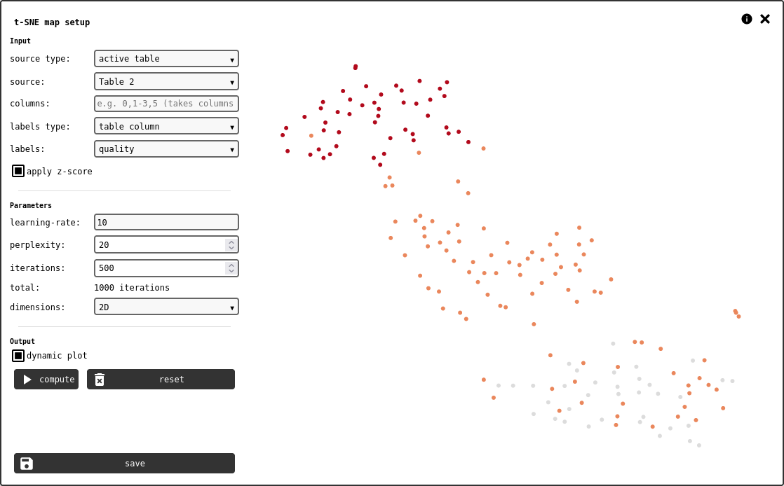
t-SNE element configuration panel.
The calculation requires any kind of matrix-like data, and optionally a vector with labels. The data should be organised so that each row of the matrix describes one data point. The data source is defined by the following controls:
source type: [selector] type of data source, either Active Table Element or DATA2D record
source: [selector] possible sources of the chosen type
columns: [text] specifies which columns of the source to use
apply Z-score: [checkbox] determines whether to apply Z-score to the source data prior to t-SNE calculation
Note
Column specifications include single indexes (i) and/or ranges (i-j), separated by comma. Indexing starts from 0, and the end index of a range is excluded. Leave blank to include all columns. Example columns specifications: * 0,2,4 (first, third and fifth columns) * 0-10 (from first to tenth) * 1-3, 10, 15-20
Warning
A matrix row will be discarded if any entry in selected columns is missing.
Colour labels can optionally be applied to the resulting t-SNE map with the following controls:
labels type: [selector] type of data source (none, table column, or DATA1D)
labels: [selector] possible labels sources of the chosen type
Note
Labels from a table column can only be used if the main data source is an Active Table Element. In such case, the same table must be the source of both data and labels.
Note
When source and labels are from the same Active Table Element, the label column is automatically excluded from the data source selection, even if explicitly listed in the column selector.
Data points with missing labels will be displayed as empty black squares, while labelled ones will be colored circles.
The following parameters determine how the t-SNE calculation is done:
learning-rate: [number] convergence accelerator
perplexity: [number] number of expected neighbours for each point
iterations: [number] number of iterations to compute
dimensions: [selector] dimensionality of the output map (2D or 3D)
dynamic plot: [checkbox] if true, the notebook will calculate t-SNE on-the fly and display an interactive plot, otherwise the system will create a static plot.
Note
Dynamic plots will make the notebook recompute t-SNE each time it is refreshed.
The calculation is then started with the compute button, which performs the desired amount of iterations on the source data. If pressed again, the system will perform additional iterations, adding up to the total indiated in the interface. The control panel records the total amount and uses it to recompute t-SNE when the notebook is refreshed if dynamic plot is chosen.
The output matrix of t-SNE calculation has one row for each valid data point and 2 or 3 columns (depending on chosen output dimension), and will be stored as a DATA2D record in the notebook, along with a DATA1D record listing the indexes of the valid rows of the source data matrix.
Python Script
The Python script element brings custom user code into the notebook. With custom scripts, it is possible to process existing data records and store the results into new records.
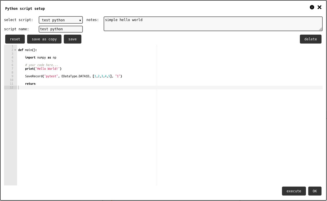
Python element configuration panel.
The configuration panel (![]() ) shows the list of all scripts available to the user; these are taken from all notebooks the user can read. The list also shows an option for starting a new script.
) shows the list of all scripts available to the user; these are taken from all notebooks the user can read. The list also shows an option for starting a new script.
The reset button clears the script code and restores the default one.
After editing the code, the script should be saved with the save button prior to execution. Alternatively, it is possible to save a new copy of the script with the save as copy button.
Warning
Saving a script will change the code globally. Every python element using the script will be affected.
The delete button will remove the script completely from the platform.
Warning
AMAD will not check if the script is used when deleting it. This might disrupt some workflow, so always make a copy of someone else’s script when using them.
Once the script is setup, the user can request its execution with the execute button, also found in the python element toolbar (![]() ). This will submit a job to a server side queue.
When the execution is completed, the element will show the results with the script stdout and eventual stderr.
). This will submit a job to a server side queue.
When the execution is completed, the element will show the results with the script stdout and eventual stderr.
Warning
Python scripts are not meant to replace local supercomputing resources! Depending on the deployment hardware specs, computing resources may be quite limited in terms of memory and CPU power. These are intended to perform custom, quick processing on reasonable size data, for example subtracting and normalising arrays/matrixes or compute their FFT.
Please read the Scripting Guidelines to found out more about the built-in scripting capabilities of AMAD
 Scanning Probe Microscopy
The SPM element can be used to import image data from scanning probe microscopes, and perform basic slope removal operations.
Different format are supported. Nanonis SXM, Brucker IBW and CreaTec DAT files are uploaded through the upload tab. This works similarly to other upload interface: drop the files in the designated area, select the ones to parse and their format, and finally upload to the server.
Omicron Matrix files have a dedicated upload MTRX tab. The user needs to provide the master file with name ending in _0001.mtrx, and all other .mtrx files with the scans. The system will create multiple SPM data records, each including all traces (up/down/forward/backward) for all channels, that are parsed from .mtrx files with same sample_name, data_set_name, session and cycle.
Scripting Guidelines
Scripts are small custom programs meant to perform operations not available in other AMAD steps. Currently only server-side python scripts are implemented.
A python script has to define a main function in order to work:
def main():

        # do something here...

        return 0
For python scripts, the return value of main will be printed in the notebook element content, thus it should be serializable data (integer, string, …). Matplot scripts should return the matplotlib pyplot object that is to be rendered in the element. Anything printed to the screen using the python print function by either script type will also be reported in the corresponding notebook element.
Note
Due to security reasons, the script cannot import certain python modules that can be harmful to the system (os, sys). The user can import other modules that are available on the system where AMAD is installed: numpy, scipy, pillow and standard packages are present.
All scripts can read the data records in the notebook using the following built-in functions:
# returns all record names in a list
names = GetRecordNames()

# fetches the record named 'some name here' from the database
rec = GetRecord('some name here')

# get the actual data
recordData = rec['data']
Records are python dictionaries, thus all the information are retrieved (data, timestamps, metadata, …): the actual data is in the data field of the dictionary, as shown in the code example.
Python scripts (not matplot) can create data records and store them in the notebook with the following built-in function:
# datatype = EDataType.DATA1D or similar
SaveRecord(name, datatype, data, units="1")
There is no limit on the amount of records that a python step can generate, but it is important to remember than record names must be unique. The units argument is optional, but recommended if the data is intended to have physical units (see Physical Quantities). The datatype argument must be a member of the built-in enum EDataType listed in this table.
Warning
The data argument must match the specified type. The system will probably not save the record correctly into the database if the type is not correct.